1 Introduction
1.1 Forecasting of electricity demand
Power load forecasting remains one of the fundamental business problems faced by the electricity sector. In particular, accurate forecasts are needed when setting up contracts between providers and consumers of electricity. If the delivered power is lower than the demand, the provider makes a loss (e.g. pays a penalty). On the other hand, when delivered power is higher than the actual demand, the provider may bear additional costs too (e.g. costs concerning selling energy on the SPOT / balancing market). Hence, the more accurate energy load forecasts, the lower costs.
Certainly, there are many kinds of energy contracts. Some of them require paying fees only when the delivered power falls below the contracted value by a certain amount. Other contracts transfer all the risk to the clients, and oblige them to buy additional energy they need on the balancing or SPOT market. Different types of contracts undoubtedly require different forecast evaluation schemes.
Choosing appropriate forecasting models that take into account specificity of electricity demand is not an easy task. Firstly, demand patterns can differ markedly. While some of them exhibit strong and usually complex seasonal behaviour, others may be quite dissimilar (e.g. without significant seasonal fluctuations). Secondly, different clients may use different time intervals to measure energy demand (in particular, not all clients have hourly registered demand). Moreover, there is a number of exogenous factors (e.g. factors related to weather conditions etc.) that may significantly influence the actual energy consumption.
1.2 Task
From an energy provider’s perspective, the main task is to construct accurate forecasts of daily or hourly electricity demands, usually for a substantial number of diverse demand patterns. Unfortunately, in practice, weak forecasting models are often used which may lead to over- or underestimated forecasts. Additionally, the applied software solutions are often not stable either. Therefore, there is a substantial need for an effective and transparent software tools being able to make energy load forecasts for many clients.
1.3 Solution
In order to provide accurate forecasts of the electricity load one has to develop a suitable approach, taking into account all specific circumstances. Of course, historical energy demand data as well as actual information concerning important external factors should be taken into account first. When building forecasting system it is equally important to take care of archiving results and performing continuous backtesting that will allow providers to verify the quality of derived forecasts. In consequence, one may expect to reduce the costs related to over- or underestimation of the energy demand.
2 Data
2.1 Data
In the analysis, we use a dataset concerned with the load of the Polish Power System (in Polish: Krajowy System Energetyczny or KSE). The original data consisting of 15 min. temporary values (in MW) were downloaded from the PSE S.A. website, and then aggregated to hourly values. Finally, we obtained over 120.000 observations containing hourly power demand values from 13 years.
Our dataset is shown in Figure 1 (note that for the sake of clarity only a selected time period is shown). It is easily seen that data exhibit multiple seasonalities, i.e.: daily, weekly, and yearly seasonal patterns can be identified. Additionally, one may observe that holidays influence the volume.
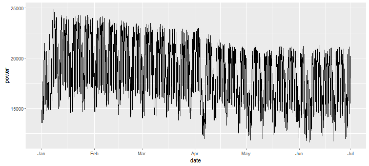 Figure 1. Hourly data containing the load of the Polish Power System in a selected time period.
2.2 Data — factors
External (exogenous) factors related to weather conditions were taken into account in the analysis as well. This included hourly data on temperature, cloud coverage and wind speed (components of the chill factor) from 82 stations from around Poland. Meteorological data were aggregated to country-level averages before analysis.
Figure 2 shows external factors registered for consecutive time points. Of course, one may expect that using this additional information may improve energy demand forecasting accuracy.
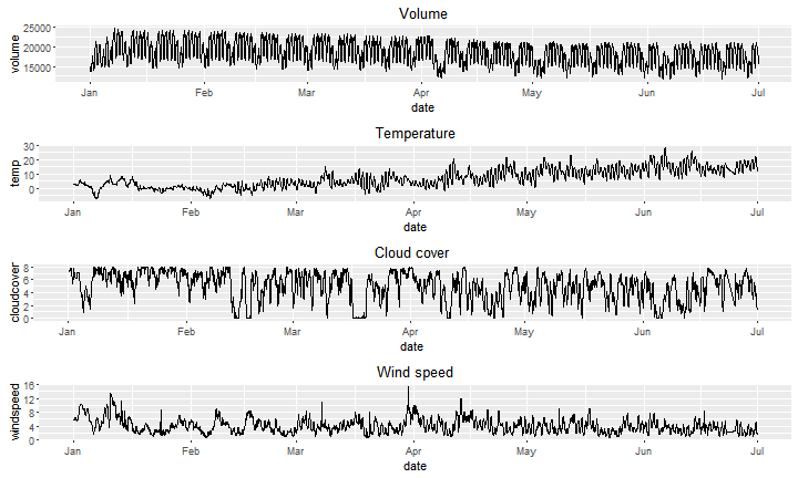 Figure 2. Daily energy load (top figure) and three external factors (related to weather conditions) that may influence energy consumption.
3 Analysis
3.1 Three approaches / frameworks
As mentioned, in order to build forecasting models we used three different approaches, proposed by three data scientists (co-authors of this report, i.e. Artur Suchwałko, Tomasz Melcer, Adam Zagdański) with different backgrounds and experience. This included:
regression modelling framework,
time series models,
deep neural networks.
Consecutive approaches will be described in more detail in the following sections. Here let us only mention that in each of the approaches different model selection methods have been tested, including both expert and data-based solutions. What is important, we assume that the forecast of the exogenous factors is perfect. It means that we do not include uncertainty of forecasting of the factors like weather into the analysis of the forecasting error. Furthermore, the standard learning-test split scheme was applied in order to compare forecast accuracy of all procedures considered in the study.
3.2 Other applications
It is worth mentioning that modelling frameworks we used in this study are quite general, and their possible applications are not limited to forecasting energy demand. In particular, described methods can be useful in forecasting other phenomena or quantities, when either external (exogenous) factors or complex seasonality patterns are present.
3.3 Regression
3.3.1 Idea
Regression analysis is a process of estimating relationships among variables. The primary goal of regression is describing (forecasting) value of a variable (called dependent) basing on values of a number of other variables (called independent).
The relationship can be described using a variety of approaches, ranging from very simple linear functions (so-called linear regression) to large non-parametric models (e.g. gaussian processes, neural networks). These methods might come both from the classical statistics/probability theory, involving mathematical models of data, and machine learning, more focused on predictive power. The choice depends on many factors. Dataset size is one of the most important factors: big datasets are required for complex methods with many degrees of freedom, where small datasets lead to overfitting. Complex methods are also usually difficult to interpret, whereas simpler methods with low number of parameters are easier to understand. However, complex methods often produce more accurate forecasts. Some other factors that influence the choice of regression method are field-specific practice (some fields settled on using a set of methods well known in the community), robustness to anomalies and violations of model assumptions, availability of specific error measures (whether it is simple to incorporate unusual criteria into the model optimization process), and computational overhead (some methods require lots of time or dedicated hardware for good results).
There is no single best approach. It is possible to compare predictive power of various approaches for a specific dataset using a variety of model selection and validation techniques, but the results will be different for different classes of datasets. Moreover, other factors might be more important to the investigator than just having accurate forecasts: for example, an interpretable model might lead to insights regarding the modeled process, and low computational overhead might be vital for short-term forecasts.
For an overview of classical and modern regression methods see e.g. Hastie, Tibshirani, and Friedman (2009)
3.3.2 What we chose?
After a couple of preliminary tests we decided to make use of classical SVM (Support Vector Machine) method. As independent variables were used volume and other factors from the present and past moments plus seasonality describing variables encoded as dummy variables. The dependent variable was volume from a future moment.
3.3.3 Forecasting with regression
Figure 3 illustrates regression approach to forecasting. It shows past values of the factors (denoted by F(⋅) ) from moments t-h to t+1 (future values are treated as known, not forecasted) and past values of the volume denoted by V(⋅) from moments t-h to t . These values form a vector of independent variables. The independent variable is the volume value from time t+1 . Regression function is denoted by f(⋅) .
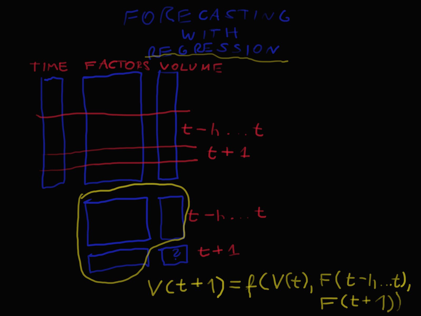 Figure 3. Forecasting with regression.
3.3.4 Variables encoding
Figure 4 shows encoding of qualitative variables like a day of a week or a calendar month. It is a classical approach when a variable having n levels is represented by n-1 of binary variables. These binary variables are known as dummy variables.
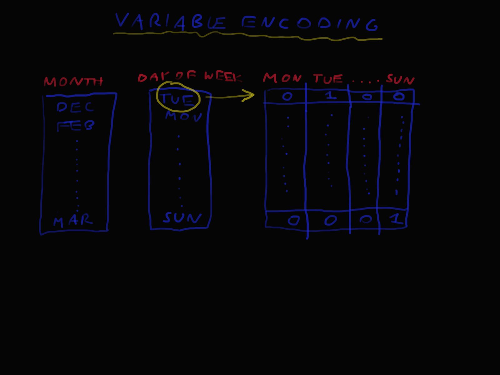 Figure 4. Idea of variable encoding in regression model.
3.3.5 Cross validation
An ordinary cross-validation relies on spliting data into a number of folds and next learning and testing of the model this number of times.
This approach with a plain random split will not work since a test set will not always lie after a learning set on the timeline. This is important for simulating real-life testing of time series forecasting models. In this situation usually a model is built on a dataset from a time period and tested on data from a next time period.
Figure 5 shows an approach to cross validation specific to time-dependent data.
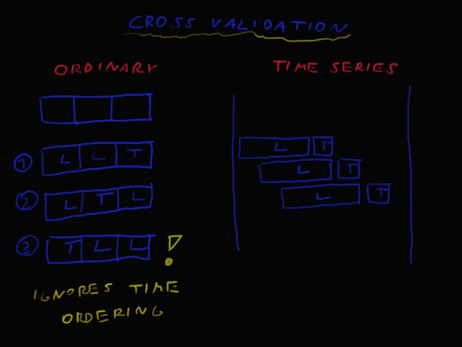 Figure 5. Idea of cross-validation scheme.
3.4 Time series models
3.4.1 Idea
Time series models were developed in order to directly incorporate a specific time-dependent structure in the analysed data. Models for time series data can have many forms (see e.g. Hyndman and Athanasopoulos (2013) or Zagdański and Suchwałko (2015)). This included but is not limited to the well-known ARMA, ARIMA, GARCH and other classes of models whose properties have been carefully studied in the vast literature. Of course, there are models devoted to time series data exhibiting complex seasonality patterns too.
Time series models are regarded as both simple and stable mathematical models, with solid theoretical basis. Such models are usually easy to interpret too. What’s more, in addition to point forecasts, prediction intervals can be constructed to indicate the likely uncertainty in point forecast. On the other hand, expert knowledge and sufficient experience are often required to find the optimal model. Another limitation is a relatively small flexibility, e.g. most of the popular classes of time series models rely on the assumption of linear dependence which may neither be adequate nor optimal for some applications.
3.4.2 What we chose?
In our analysis, we use classical harmonic (or Fourier) regression with additional regressors (factors) and ARMA errors. In this case, multiple seasonality is modelled with the aid of Fourier series with different periods, i.e. appropriate combinations of sine and cosine functions (called harmonic components). Additionally, external factors (e.g. temperature, wind speed, etc.) can be easily included in the model. Short-term time correlation is modelled using well-known ARMA models. For the sake of simplicity, the lagged factors were not included in the final model.
3.4.3 Modelling complex seasonality via harmonic regression
Figure 6 shows seasonal components obtained on the basis of harmonic regression model. This includes daily, weekly as well as annual seasonality.
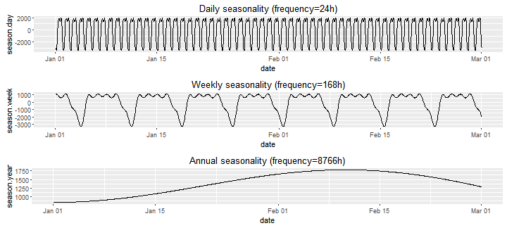 Figure 6. Seasonal components in energy load data obtained on the basis of harmonic regression model.
For illustrative purposes, in Figure 7 we also show estimated harmonic (Fourier) terms, whose linear combination is used to capture annual seasonality in the fitted model. Note that five pairs of harmonic components are shown, and this number can be further optimized to improve forecasting accuracy. Certainly, analogous harmonic terms were obtained for weekly and daily seasonality (results not shown).
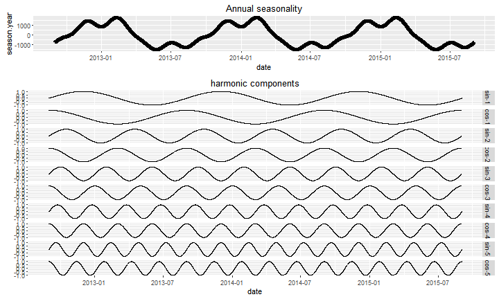 Figure 7. Harmonic components for annual seasonality.
3.5 Deep neural networks
3.5.1 Idea
Deep learning is a branch of machine learning that considers a class of models initially studied as models mimicking biological neural networks. Thanks to the algorithm of backpropagating errors, availability of massively parallel computating hardware in form of GPUs, and large datasets becoming common, deep learning recently became quite popular.
Deep learning covers a variety of models useful for a number of cognition-related tasks, such as image object recognition or natural language processing, as well as analysis of more abstract concepts like time series. The models are easy to scale upwards to provide more learning capacity, necessary to take advantage of large datasets. The recent breakthroughs drove many large tech companies to publish open-source libraries dedicated to deep learning.
However, deep learning models are often very difficult to interpret due to a large number of parameters, inherent complexity and lack of substantial mathematical understanding. Moreover, the models are extremely easy to overfit, and hence not a good fit for small datasets. Additional hurdle is that these methods are often computationally demanding, requiring expensive hardware for efficiency.
3.5.2 What we chose?
We constructed a standard feed-forward network that learns a mapping of date, time, power demand and weather conditions of a single hourly period to power demand during the subsequent hour. The overall structure is shown on figure 8.
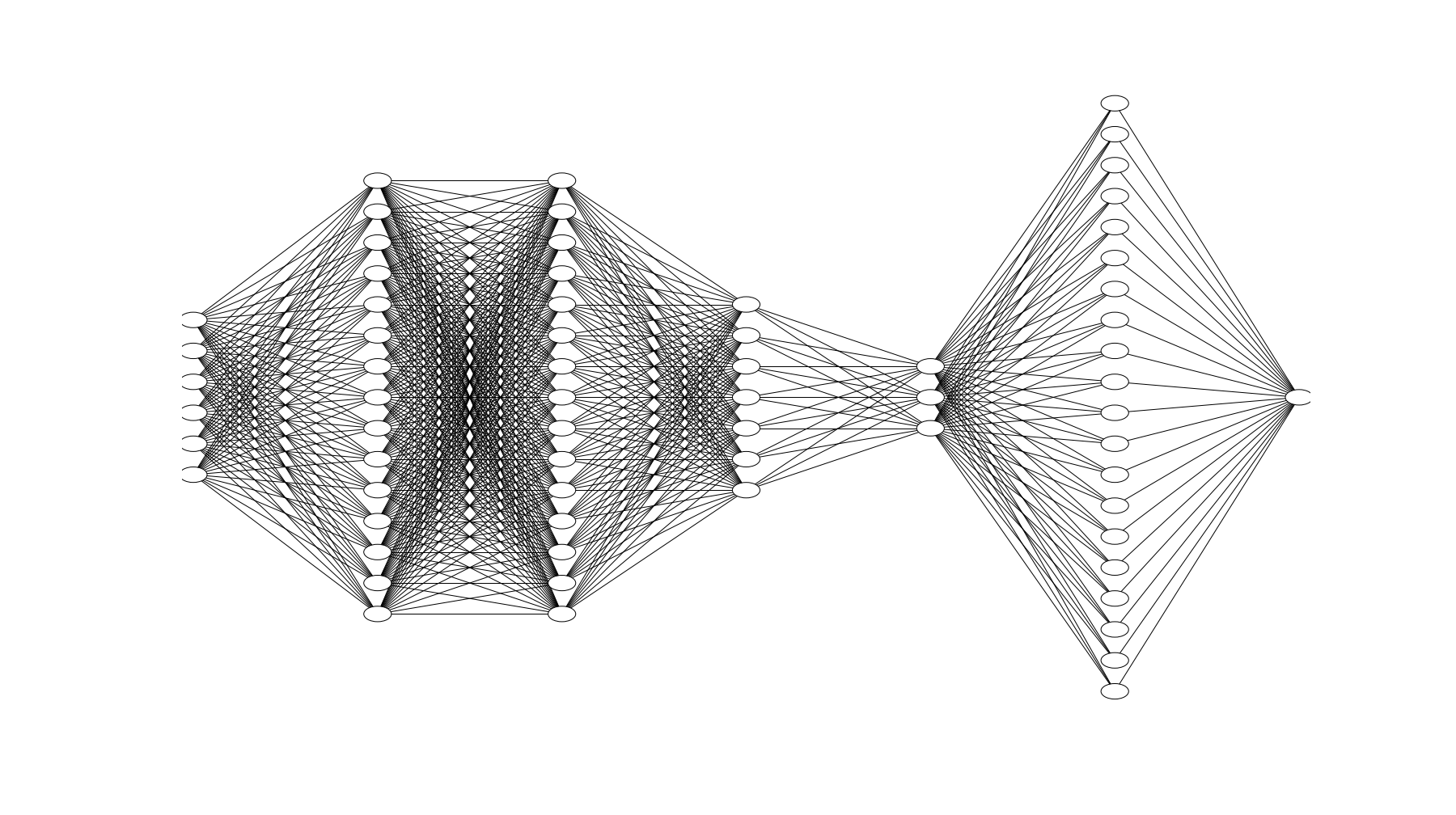 Figure 8. Neural network structure.
The input layer takes a vector of 112 input values, where month, day of month, day of week, hour and weather data were passed as dummy-encoded variables. The input layer passes data to a stack of four fully-connected hidden layers of 256, 256, 64 and 16 neurons each. Each of these layers uses the tanh activation method and dropout. The next layer consists of 817 neurons with the softmax activation method. The layer encodes the probability distribution of the predicted value. Each neuron in this layer represents a belief that power demand for the next hour will fall into a specific interval of length 20 MW. To drive the optimization procedure into this representation, a single output neuron with fixed weights was attached to this layer to compute expected value of this probability distribution. The full network uses 126.097 model parameters in all layers.
To train the model we used Stochastic Gradient Descent algorithm with Nesterov momentum, with MAPE of the single output neuron as an error measure. Training was stopped after 1.000 epochs with no improvement in error measure on a validation dataset.
3.6 Aggregating of forecasts
3.6.1 Idea
Ensemble learning has been successfully used in statistics and machine learning for a few decades already (see e.g. Hastie, Tibshirani and Friedman (2009)). Roughly speaking, the main idea of such approach is to combine (aggregate) results from multiple learning algorithms in order to obtain better predictive performance. Significant diversity among the models (committee members) usually yields better results.
Similar procedure can be utilized in the context of forecasting time-dependent data too. One can expect that combining forecasts will result in the superior performance over the use of individual model. Certainly, there are different averaging schemes, including: simple averaging, weighted averaging (weights assigned to individual forecasts according to their accuracy), as well as different variants of regression models (individual forecasts are used as regressors).
3.6.2 What we chose?
In our analysis a simple averaging scheme has been used, i.e. the most natural approach to combine forecasts obtained from three different models. The arithmetic mean of all forecasts produced by the individual models were computed. Note that despite its simplicity such approach is highly robust and widely used in business and economic forecasting.
4 Results
4.1 Prediction errors (backtest)
In the context of energy forecasting, it is common to consider short-, medium- or long-term forecasts (see e.g. Weron (2006)). On the other hand, there is no consensus in the literature what actual forecasting horizon ranges constitute each of these forecast classes, hence it remains problem-dependent.
In order to carefully investigate the performance of all models we decided to compare hourly forecasts for three horizons: 60, 120, and 360 days (recall that each day correspond to 24 time points). It is worth pointing out that hourly forecasts are constructed rather for shorter horizons, and when long-term forecasts are needed low frequency data can be utilized (e.g. daily instead of hourly). We used the standard MAPE (Mean Absolute Percentage Error) as a measure of out-of-sample (test set) forecast accuracy. Certainly, other accuracy measures for forecast models could be used too, depending on the business goal, etc.
Table 1 contains MAPE forecast errors obtained for all approaches considered in our analysis, i.e. time series model, regression, deep neural network and simple average of these three forecasts. Additionally, as a reference result we used forecasts obtained basing on the seasonal naive method, i.e. the energy load values from the last day are used as forecasts for the next periods (days). Using naive methods as benchmarks in forecasting is important. Energy demand data often exhibit high level of average volume and relatively small magnitude of seasonal changes. In the presence of them naive forecast may perform surprisingly well. Obviously, usability of these forecasts is not very high.
4.2 History and three forecasts
Figure 9 shows three time series. Each of them consists of historical energy load values followed by forecasts obtained from a particular method.
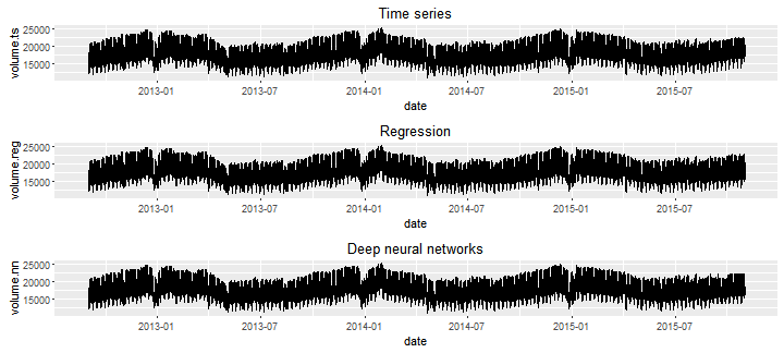 Figure 9. Historical data and forecasts — comparison of results.
We intentionally left the limit between history and forecast non-marked. Thanks to this we can see that all the methods can reflect seasonality in the forecasts. Generally speaking, all the forecasts make sense.
4.3 More detailed comparison of the forecasts
Figure 10 allows us to compare all forecast approaches in more detail.
 Figure 10. Comparison of forecasts for all methods.
Figure 11 shows a detailed comparison of the forecasts for a selected week. We can clearly see that none the methods were able to predict a volume drop on 11th of November, a national holiday in Poland.
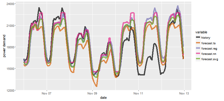 Figure 11. Comparison of forecasts for a selected week.
We can see that there are substantial differences between the forecasts, e.g. that some of methods systematically underestimate and some overestimate. This behavior of methods can be corrected using non-standard error criteria, e.g. including penalty for over- or underestimation.
4.4 PDF approximation by neural networks
Our deep learning model’s next to last layer was an attempt to produce a probability distribution over the range of output values. Figure 12 presents example valuations given by the network to this layer for two data points. We observe that while sometimes the network has a strong belief towards a small range of values, there are also cases when the belief is spread over a wider range with little indication as to which value is more likely.
Having access to detailed probability distribution of predictions is useful when in order to make the best decision regarding power prediction from a financial point of view one needs to take contract details into account.
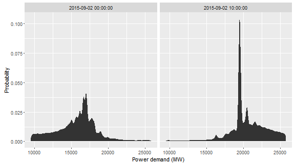 Figure 12. Probability density function approximation using neural network.
5 Toolbox
5.1 SYNOP reports
Weather data were collected from OGIMET, a free weather information service. Data are provided in form of SYNOP reports. Parsing SYNOP data is a non-trivial task: the format is not one of commonly used. It’s a text format, where information is encoded in numbers with semantics defined by both numeric value and position. Moreover, some reports do not conform to any documentation we could find, likely because the reports contained transcription errors.
OGIMET contains data starting from 2000. Poland is covered by 82 stations. Each station’s data have missing values. The holes can be as small as few hours and as large as years. Data are usually reported once an hour, however there are records deviating from this pattern.
SYNOP reports for Poland were downloaded using a custom Python script that took care of various limitations of the OGIMET API service, including strict limits on frequency and size of requests. The reports were parsed and converted into a data frame using GNU text utils. Further preprocessing was done in R using the dplyr package. For simplicity, we dropped 500 records that were not reported on the hour. Data for each hour was aggregated over all stations that reported in a given hourly period. Weather time series had to be aligned to historical power demand data series.
5.2 Regression
We used R statistical environment powered by an excellent caret package. To choose from many parameters feasible we applied grid parameter tuning with cross-validation.
The task of estimation and assessment of the models can be resource-consuming. Parallel processing was important to complete it in a reasonable time. Additionally, performing the analysis required doing some tricks to speed up the calculations.
5.3 Time series models
In order to fit time series models we used R statistical environment and some tools available in the seminal forecast package (library). Taking into account data size, to reduce computational burden some built-in parallel processing was employed to find the best ARMA model. Original data were only slightly preprocessed before actual model fitting, i.e. temperature was transformed with the aid of classical polynomial transformation in order to handle nonlinear dependence.
5.4 Deep neural networks
Deep learning algorithms were run on an NVIDIA GeForce GTX 960 graphics card. The model was defined in Python, using Keras deep learning library with Theano backend. Additional preprocessing was performed using Jupyter and Pandas. The final model required about 1 hour of computations for convergence.
6 Summary
Finally, it is time to briefly summarize our results.
First, we attempted to show that similarly as with other analytical tasks, electric power load forecasting can be accomplished in many ways, including both better and worse ones. Of course, selection of an optimal approach depends on the business goal, expectations as well as on the experience of a data analyst. On the one hand, there are no methods that are universal and optimal for all applications, and forecasting energy demand is just one example of such situation. On the other hand, you often do not have to use sophisticated methods to perform the task well enough.
As it was expected, all advanced approaches uniformly (i.e. for all considered forecast horizons) outperformed the simple seasonal naive method that was used as a reference procedure. The overall best results were obtained for deep neural network models being the most flexible approach included in our study. However, their significant limitation may be lack of interpretability as well as computational burden required to learn a final network.
The efficiency of a given forecasting approach usually depends on many factors, including regularity or irregularity of energy demand patterns, the presence of temporary changes related to holidays or weather conditions within a given time period, etc. Therefore, it is always highly recommended to carefully evaluate the performance of a given forecasting algorithm with the aid of a backtesting scheme.
A simple aggregation (or averaging) of forecasts obtained from different procedures may or may not yield better accuracy, though it is definitely worth considering when a few diverse forecasting procedures are employed.
All of these forecasts in the three frameworks can be improved, e.g. by using more sophisticated variables describing factors, playing with depth of historical data (window) we use for forecasting, using other methods or doing more careful parameter selection.
Custom optimization criteria reflecting terms of a contract between the provider and the consumer can be used, e.g. greater penalty for underestimation than for overestimation of the future volume.
Despite general lack of interpretability, it is possible to provide PDF-based estimates in neural network models. However, convergence of these models is a problem.
None of the methods predicted lower demand during fixed-date national holidays. While some methods might not be expressive enough to memorize these events, the neural network’s model structure was designed specifically to allow the network to express relations necessary to adjust predictions for these periods.
Last but not least, one should keep in mind that minimizing forecast error is not a solution for everything! There are other important issues in practical forecasting such as: model’s interpretability, controlling of model risk and stability, having full control of the forecasting process, continuous monitoring of the model’s performance etc.
Selection of the best methods depends on these factors, not only on the forecast error.